 羽落天青 | Uke's Blog

1305 字
7 分钟
人工智能通识的第一次作业
为展现PCA,kPCA与谱聚类等经典机器学习算法在人脸识别上的应用,我们选取了Olivetti人脸数据集进行分析,采用控制变量法,对PCA->kmeans,KernelPCA->kmeans,PCA->谱聚类,KernelPCA->谱聚类四种方法进行对比分析,并使用ARI与NMI两种方式评估结果。
导入olivetti数据集,并导入numpy、sklearn、matplotlib库,设置可视化模板,给出所有可视化函数
import numpy as npimport matplotlib.pyplot as plt#这里我们导入了一个好看的模板plt.style.use("seaborn-v0_8")
plt.rcParams.update({ "figure.dpi": 140, "savefig.dpi": 300, "font.size": 18, "font.family": "sans-serif", "font.sans-serif": ["Microsoft YaHei", "DejaVu Sans"], "axes.titlesize": 13, "axes.labelsize": 11, "axes.unicode_minus": False, "axes.spines.top": False, "axes.spines.right": False, "axes.grid": True, "grid.alpha": 0.25,})from sklearn.datasets import fetch_olivetti_facesfrom sklearn.preprocessing import StandardScalerfrom sklearn.decomposition import PCA, KernelPCAfrom sklearn.cluster import KMeans, SpectralClusteringfrom sklearn.metrics import adjusted_rand_score, normalized_mutual_info_scorefrom sklearn.metrics import confusion_matriximport seaborn as sns
#这里我们做了很多个可视化函数def show_distinct_people(images, labels, max_people=40): unique_ids = np.unique(labels) n_show = min(max_people, unique_ids.size) cols = 8 rows = int(np.ceil(n_show / cols)) fig, axes = plt.subplots(rows, cols, figsize=(2.2 * cols, 2.3 * rows)) axes = np.array(axes).reshape(-1)
for i, person_id in enumerate(unique_ids[:n_show]): idx = np.where(labels == person_id)[0][0] axes[i].imshow(images[idx], cmap="gray") axes[i].set_title(f"id:{person_id}") axes[i].set_xticks([]) axes[i].set_yticks([])
for ax in axes[n_show:]: ax.axis("off")
fig.suptitle(f"不同身份人脸总览 ({n_show}/{unique_ids.size})", y=1.02) plt.tight_layout()
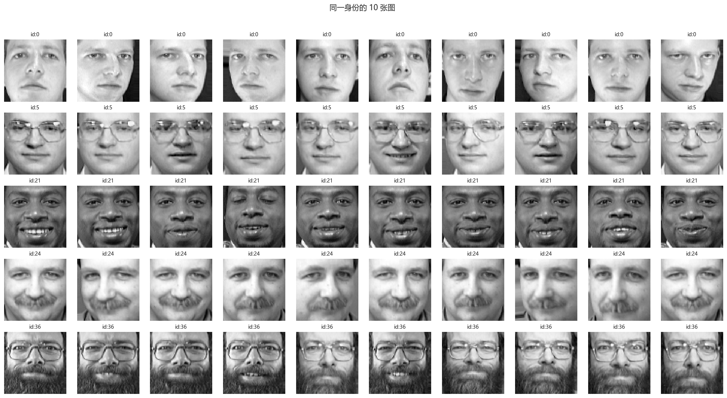
def show_10_faces_of_subjects(images, labels, subject_ids): cols = 10 rows = len(subject_ids) fig, axes = plt.subplots(rows, cols, figsize=(1.8 * cols, 1.9 * rows)) axes = np.array(axes).reshape(rows, cols)
for i, subject_id in enumerate(subject_ids): idx = np.where(labels == subject_id)[0] if idx.size == 0: continue for j in range(cols): use_idx = idx[j % idx.size] axes[i, j].imshow(images[use_idx], cmap="gray") axes[i, j].set_xticks([]) axes[i, j].set_yticks([]) axes[i, j].set_title(f"id:{subject_id}", fontsize=9) fig.suptitle(f"同一身份的 10 张图 ", y=1.02) plt.tight_layout()
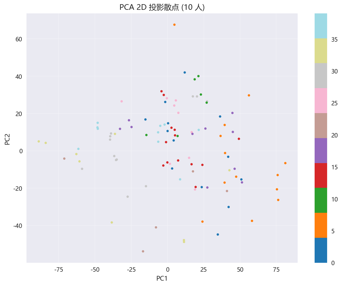
def plot_pca_embedding(Z, labels, n_people=10): n_points = min(Z.shape[0], n_people * 10) fig, ax = plt.subplots(figsize=(9, 7)) sc = ax.scatter( Z[:n_points, 0], Z[:n_points, 1], c=labels[:n_points], s=14, cmap=plt.get_cmap("tab20", n_people), ) ax.set_title(f"PCA 2D 投影散点 ({n_people} 人)") ax.set_xlabel("PC1") ax.set_ylabel("PC2") fig.colorbar(sc, ax=ax) plt.tight_layout()
def plot_explained_variance(model_pca): ratio = model_pca.explained_variance_ratio_ cum_ratio = np.cumsum(ratio) fig, axes = plt.subplots(1, 2, figsize=(12, 4.5))
axes[0].plot(ratio, lw=1.8) axes[0].set_title("主成分方差比") axes[0].set_xlabel("Component") axes[0].set_ylabel("Explained variance ratio")
axes[1].plot(cum_ratio, lw=2) axes[1].axhline(0.9, ls="--", lw=1.2, color="tab:red", label="90%") axes[1].set_title("累计方差比") axes[1].set_xlabel("Component") axes[1].set_ylabel("Cumulative ratio") axes[1].legend() plt.tight_layout()
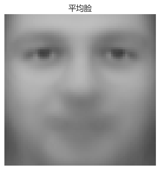
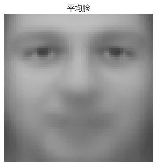
def plot_mean_and_eigenfaces(model_pca, scaler, image_shape=(64, 64), n_show=20): fig, ax = plt.subplots(1, 1, figsize=(4, 4)) # PCA is fitted on X_std, so map mean back to pixel space for human-readable visualization. mean_face = scaler.inverse_transform(model_pca.mean_.reshape(1, -1)).reshape(image_shape) mean_face = np.clip(mean_face, 0.0, 1.0) ax.imshow(mean_face, cmap="gray", vmin=0.0, vmax=1.0) ax.set_title("平均脸") ax.set_xticks([]) ax.set_yticks([]) plt.tight_layout()
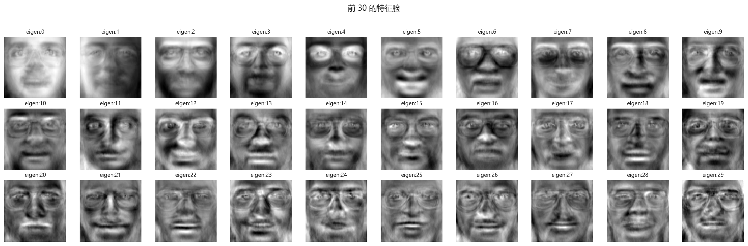
n_show = min(n_show, model_pca.components_.shape[0]) cols = 10 rows = int(np.ceil(n_show / cols)) fig, axes = plt.subplots(rows, cols, figsize=(1.8 * cols, 1.9 * rows)) axes = np.array(axes).reshape(-1) eigen_faces = model_pca.components_.reshape((-1, image_shape[0], image_shape[1]))
for i in range(n_show): axes[i].imshow(eigen_faces[i], cmap="gray") axes[i].set_title(f"eigen:{i}", fontsize=9) axes[i].set_xticks([]) axes[i].set_yticks([]) for ax in axes[n_show:]: ax.axis("off")
fig.suptitle(f"前 {n_show} 的特征脸", y=1.02) plt.tight_layout()
def plot_cluster_confusions(y_true, pred_dict, n_classes): fig, axes = plt.subplots(2, 2, figsize=(12, 10)) axes = axes.ravel() labels = np.arange(n_classes)
for ax, (name, y_pred) in zip(axes, pred_dict.items()): cm = confusion_matrix(y_true, y_pred, labels=labels) sns.heatmap(cm, ax=ax, cmap="Blues", cbar=False) ax.set_title(name) ax.set_xlabel("Predicted cluster label") ax.set_ylabel("True subject id") fig.suptitle("混淆矩阵热图", y=1.02) plt.tight_layout()将数据归一化,去中心化
data = fetch_olivetti_faces(shuffle=True, random_state=0)X = data["data"]y = data["target"]images = data["images"]scaler = StandardScaler(with_mean=True, with_std=True)X_std = scaler.fit_transform(X)k = 65c = int(np.unique(y).size)seed = 0
show_distinct_people(images, y, max_people=40)show_10_faces_of_subjects(images, y, subject_ids=[0, 5, 21, 24, 36])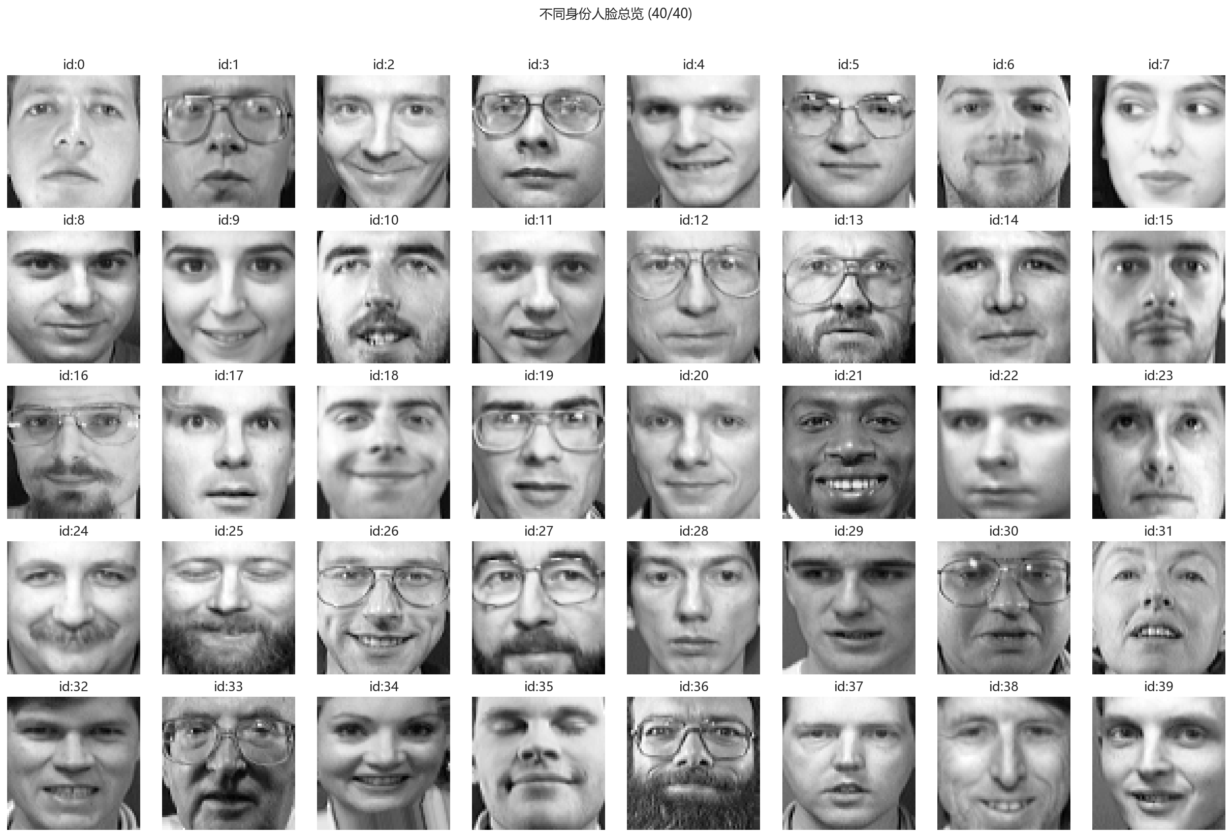
使用PCA与搭载高斯核的KernelPCA两种方式对数据进行降维,得到两种不同的主特征
pca = PCA(n_components=k, random_state=seed)Z_pca = pca.fit_transform(X_std) # (n, k)plot_explained_variance(pca)plot_mean_and_eigenfaces(pca, scaler, image_shape=images.shape[1:], n_show=30)plot_pca_embedding(Z_pca, y, n_people=10)
from sklearn.metrics import pairwise_distancesD2 = pairwise_distances(X_std, squared=True)med = np.median(D2[np.triu_indices_from(D2, k=1)])gamma0 = 1.0 / medkpca = KernelPCA(n_components=k, kernel="rbf", gamma=gamma0, fit_inverse_transform=False)Z_kpca = kpca.fit_transform(X_std) # (n, k)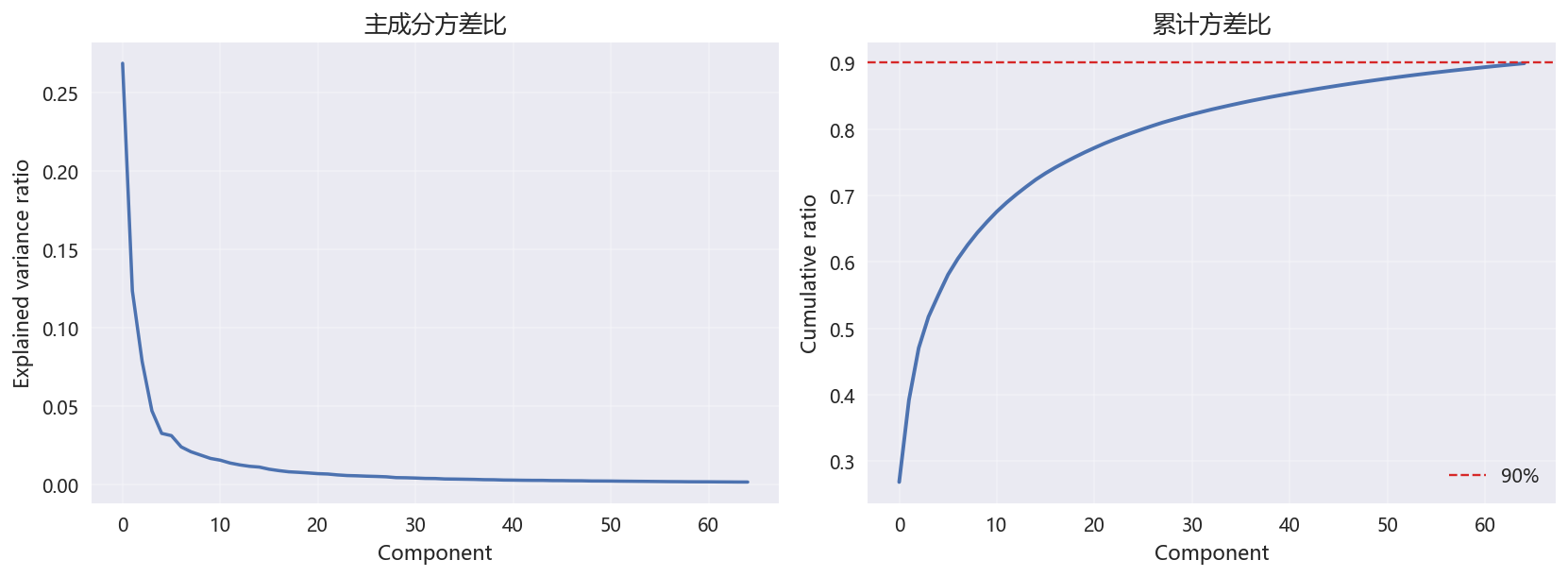
分别采用k-means与谱聚类两种方式对上述两种主特征进行聚类分析,并使用ARI与NMI两种方式评估结果
def eval_clustering(name, y_pred): ari = adjusted_rand_score(y, y_pred) nmi = normalized_mutual_info_score(y, y_pred) print(f"{name:18s} ARI={ari:.4f} NMI={nmi:.4f}")km1 = KMeans(n_clusters=c, random_state=seed, n_init="auto")y_pca_km = km1.fit_predict(Z_pca)eval_clustering("PCA -> KMeans", y_pca_km)
sp1 = SpectralClustering( n_clusters=c, affinity="nearest_neighbors", n_neighbors=10, random_state=seed, assign_labels="kmeans",)y_pca_sp = sp1.fit_predict(Z_pca)eval_clustering("PCA -> Spectral", y_pca_sp)
km2 = KMeans(n_clusters=c, random_state=seed, n_init="auto")y_kpca_km = km2.fit_predict(Z_kpca)eval_clustering("kPCA -> KMeans", y_kpca_km)
sp2 = SpectralClustering( n_clusters=c, affinity="nearest_neighbors", n_neighbors=10, random_state=seed, assign_labels="kmeans",)y_kpca_sp = sp2.fit_predict(Z_kpca)eval_clustering("kPCA -> Spectral", y_kpca_sp)
predictions = { "PCA -> KMeans": y_pca_km, "PCA -> Spectral": y_pca_sp, "kPCA -> KMeans": y_kpca_km, "kPCA -> Spectral": y_kpca_sp,}plot_cluster_confusions(y, predictions, n_classes=c)
fig, axes = plt.subplots(1, 2, figsize=(12, 5))axes[0].scatter(Z_pca[:, 0], Z_pca[:, 1], c=y_pca_km, s=10, cmap="tab20")axes[0].set_title("PCA features clustered by KMeans")axes[0].set_xlabel("PC1")axes[0].set_ylabel("PC2")
axes[1].scatter(Z_pca[:, 0], Z_pca[:, 1], c=y_pca_sp, s=10, cmap="tab20")axes[1].set_title("PCA features clustered by Spectral")axes[1].set_xlabel("PC1")axes[1].set_ylabel("PC2")plt.tight_layout()PCA -> KMeans ARI=0.4163 NMI=0.7598PCA -> Spectral ARI=0.5245 NMI=0.8088kPCA -> KMeans ARI=0.4638 NMI=0.7897
kPCA -> Spectral ARI=0.5314 NMI=0.8187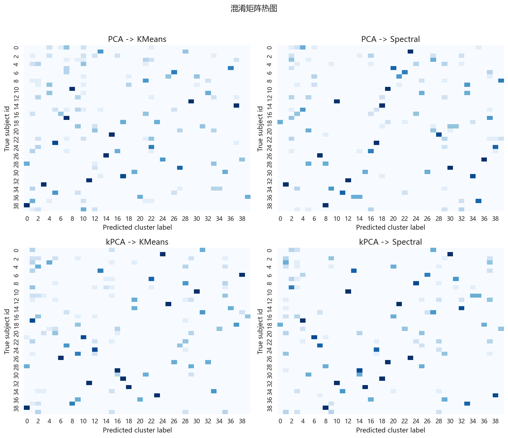
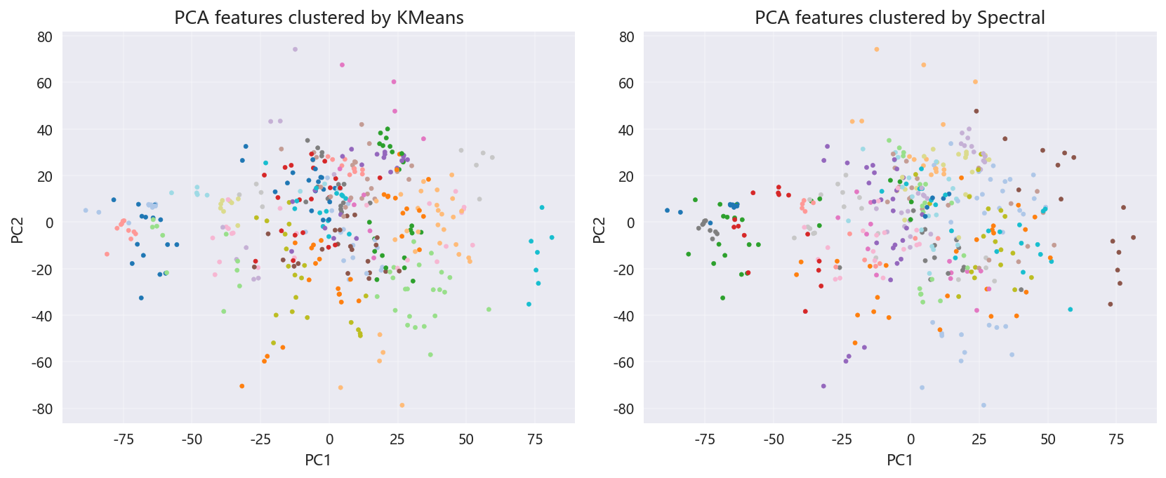
我们可以看到,PCA与kPCA两种方式得到的主特征在视觉上差异不大,但在聚类分析上,kPCA的表现明显优于PCA,说明核方法在捕捉数据的非线性结构方面具有优势。同时,谱聚类相较于k-means在PCA特征上的表现提升更为显著,说明谱聚类在处理复杂数据结构时更具适应性。
总体而言,kPCA与谱聚类的结合在本次人脸识别任务中表现最佳,说明在处理高维且具有复杂结构的数据时,非线性降维与图论方法的结合能够更有效地揭示数据的内在模式。
我想,对于小样本量的无监督学习来说,这样的ARI核NMI正确率已然不错,我们完美的完成了课堂任务,很好的运用了矩阵论知识以及机器学习算法,展现了PCA、核PCA与谱聚类在实际问题中的应用效果。